Understanding Math of Money Market: Part 2
Introduction
This is the second part of a three-part series of building a Money Market on ICE which would allow anyone to supply cryptocurrencies to earn interest as well as borrow cryptocurrencies for loans.
In the first part of the series, we introduced the parameters involved in the money market. In this part, we introduce how those parameters are calculated.
Interest Rates
As mentioned in the first part, the interest rates of the reserve can change with each transaction. So let’s talk about how it changes and how is it calculated.
Interest rates are calculated as per the utilization rate and as discussed in the first part, the utilization rate depends upon Total Liquidity (Lₜ) and Total Borrows (Bₜ).

Now that we have calculated the utilization rate, we can calculate the interest rates. Borrow interest rates (Rᵥ)can be calculated with respect to the Utilization Rate (U) by using the following formula.

In the above formula,
R_v0 = Base borrow rate
U_optimal = Optimum utilization rate that the model targets
R_slope1 and R_slope2 are constants
Now that we have Rᵥ, we can calculate liquidity rate (supply rate) Rₗ by multiplying Rᵥ with U.

Note: Liquidity and supply are used interchangeably.
To further strengthen our understanding, let’s plot how the interest rate changes with the utilization rate. Let’s set our variables as
R_v0 = 2%
U_optimal = 0.8
R_slope1 = 6
R_slope2 = 1

In the above graph, the red line represents the borrow interest rate and the green line represents the supply interest rate.
We get a lot of insights from the graph including:
- The supply rate is always less than the borrowing rate.
- The borrow rate is linear but the supply rate seems to be quadratic. This can be easily seen from the formulas. Borrow rate is directly proportional to U. Therefore, supply rate = U * Borrow Rate ~ U * U.
- As the utilization rate increases, the borrow rate increases and so does the supply rate. Above optimum utilization rate, the difference between supply rate and borrow rate decreases faster and at U=1, Supply Rate = Borrow Rate.
Since the utilization rate is based on total deposits and total borrows, we can adjust them to see how the interest rate changes with the change in borrows and deposits as well.

Similarly, we can also adjust the constants we mentioned earlier to see how those values affect the interest rates.
We have seen that interest rate changes with the changes in the amounts of borrow and deposits. Thus to calculate the interest accrued over time, we have to consider these changes over time.
To make things simpler, we’ll be using the same case of a single reserve for all our examples and calculations. The case is described below.
Note: Supply and liquidity are used interchangeably.
At T=0, A deposits 1 token
At T=0, B deposits 2 tokens
At T=0, C deposits 2 tokens
At T=50, D borrows 1 token
At T=80, B withdraws 1 token
At T=80, C deposits additional 1 token
At T=80, E borrows 2 tokens
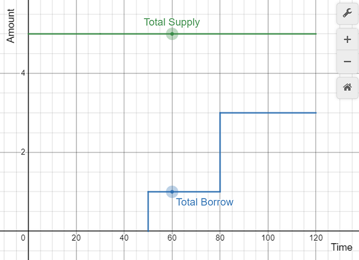
In the above figure, green line represents the total supply and blue line represents the total borrows.
It should be noted that the total supply (liquidity) has not changed over time. This is because:
Total Liquidity (Lₜ)= Available Liquidity (Lₐ)+ Total Borrows (Bₜ)
Note: The total borrows Bₜ is the actual amount borrowed plus the interest on that amount. To keep things simple for now, we ignore the interest on the borrowed amount from total borrows.
We’ll consider the interest on the borrowed amount after we have discussed about the cumulated indices and scaled amounts.
At T=0:
A supplies 1 tokens [Lₐ = 1, Bₜ = 0 ]
B supplies 2 tokens [Lₐ = 3, Bₜ = 0]
C supplies 2 tokens [Lₐ = 5, Bₜ = 0]
At T=50, t
D borrows 1 token [Lₐ= 4, Bₜ = 1]
At T=80,
B withdraws 1 token [Lₐ = 3, Bₜ= 1]
C deposits 1 tokens [Lₐ = 4, Bₜ = 1]
E borrows 2 tokens [Lₐ = 2, Bₜ = 3]
And therefore the liquidity always remained 5 throughout T=0 to T=80. Since there is no activities after T=80, we can see that the liquidity remains the same thereafter as well.
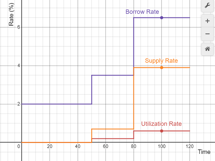
As the total liquidity Lₜ and total borrows Bₜ changes, so does the Utilization Rate U. Since the interest rate depend on U, we can see that Supply Rate ( Liquidity Rate Rₗ) and Borrow Rate Rᵥ changes as well.
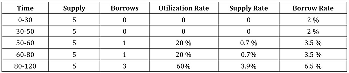
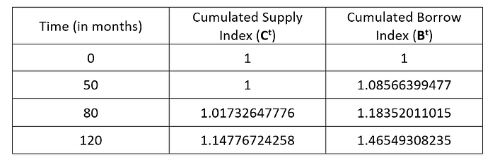
All the information is summarized in the following table.
Cumulated Index
Cumulated index combines entries from previous indexes to make the calculations faster and efficient. To build the intuition for cumulated index, we’ll try to calculate the total amount that can be redeemed by User A at T=120.
Let us represent the initial Amount supplied by User A as A₀. Since user A supplied 1 token, A₀ = 1.
Interest accrued from T=0 to T=50 [50 months]
I₁ = Interest on A₀ token at 0% for 50 months
Interest accrued from T=50 to T=80 [30 months]
I₂ = Interest on (A₀+I₁) tokens at 0.7% for 30 months
Interest accrued from T=80 to T=120 [40 months]
I₃ = Interest on (A₀+I₁+I₂) tokens at 3.9% for 40 months
Total Amount = 1 + I₁+ I₂ + I₃
Alternatively, we can also represent the total amount at different times.
Total amount at T=50
A₁ = A₀ + I1
Total amount at T=80
A₂ = A₀ + I₂
Total amount at T=120
A₃ = A₀ + I₃
We know the final amount, A after simple interest can be calculated by the formula, A = P(1 + R*t) where,
- P = Principal Amount
- t = Time duration (in years)
- R = Rate of interest
Since we are making calculations in seconds instead of the year, we first need to convert months into equivalent seconds and then divide it by no of seconds in a year to get the equivalent representation. Let’s represent no of seconds in a year by Tᵧ and no of seconds in a month by Tₘ.
Total amount at T=50 months
A₁ = (1 + R * t/Tᵧ ) 1 [R=0%, t=50 * Tₘ] (T=0 to T=50)
Total amount at T=80 months
A₂ = A₁ (1 + R* t/Tᵧ ) A₁ [R=0.7%, t=30* Tₘ] (T=50 to T=80)
Total amount at T=120 months
A₃ = (1 + R * t/Tᵧ ) A₂ [R=3.5%, t=40* Tₘ] (T=80 to T=120)
It can be noted that the total amount depends on the previous total amount.
With that in mind, let’s define the concept of cumulated index such that the multiplication of the initial principal amount with this index gives the final amount.
Liquidity Cumulated Index
For the calculation of final amount that can be redeemed after supply, we make use of the cumulated index called liquidity cumulated index. It is denoted by Cᵗ and defined as:

where
Cᵗ is the cumulated liquidity index over time t.
Rₗ is the interest rate on supply
To understand △T_year, let’s define
- T = Current number of seconds as defined by
block.timestamp - Tₗ = Last updated timestamp of the data. Tₗ is updated every time a borrow, deposit, redeem or repay event occurs.
- T_year (Tᵧ) = No of seconds in a year = 31536000
- △T_year = (T — Tₗ) / Tᵧ
Note: C⁰ = 1.
Let’s see how Cᵗ changes for the case study we have taken.
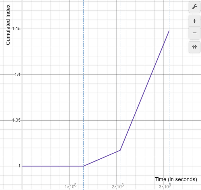
Note: In the above graph, the blue dotted lines represent the timestamp of T=50 months, T=80 months and T=120 months respectively.
The use of Cᵗ allows us to easily calculate the total amount (principal amount + interest) at any time by simply multiplying the Cᵗ with the amount deposited (principal amount).
Until time T=50, there is no interest on supply and thus multiplying Cᵗ with the deposited amount will result only the deposited amount as there is no interest.
For time T>50, we can see how the total amount changes with time.
- Between 50<T≤80, the interest rate is 0.7% and thus the amount accumulated is increasing slowly over time.
- However, between 80<T≤120, the interest rate is 3.9% and thus the amount accumulated increases sharply with time.
It should be noted that the value of Cᵗ never decreases. It can be constant over some time if the interest rate over that period is zero.
Borrow Cumulated Index
Borrow cumulated index is similar to the liquidity cumulated index in a sense that multiplying the initial principal amount with this index gives the final amount. However, the initial principal amount in this case is the amount borrowed and the final amount is the amount that needs to be repaid.
If we make use of simple interest to calculate the interest on borrows the borrow cumulated index can be denoted by Bᵗ and defined as:
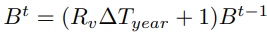
But for the purpose of this article, we will be using compound interest to calculate the interest on borrows. The final amount A after compound interest can be calculated by the formula, A = P(R/Tᵧ + 1) where,
So the cumulative index can be defined as:
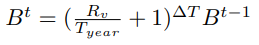
where
Bᵗ is the cumulated borrow index over time t.
Rᵥ is the interest rate on borrow
T_year (Tᵧ) is the no of seconds in a year = 31536000
△T is time duration on seconds from the last updated timestamp Tₗ
Note: B⁰ = 1.
Let’s see how Bᵗ changes for the case study we have taken.
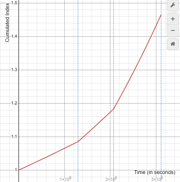
Note: In the above graph, the blue dotted lines represent the timestamp of T=50 months, T=80 months and T=120 months respectively.
For further clarity, let’s see how borrow cumulated index and liquidity cumulated index change in respect to each other.
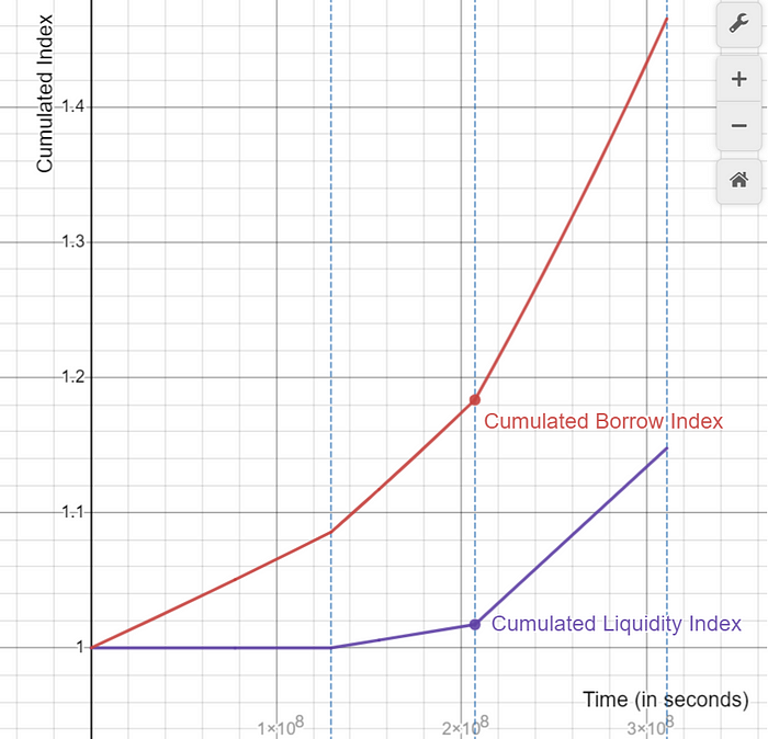
Note: Although both curves seem linear at this scale, we can extend the T in the x-axis to see the true nature of the curves.
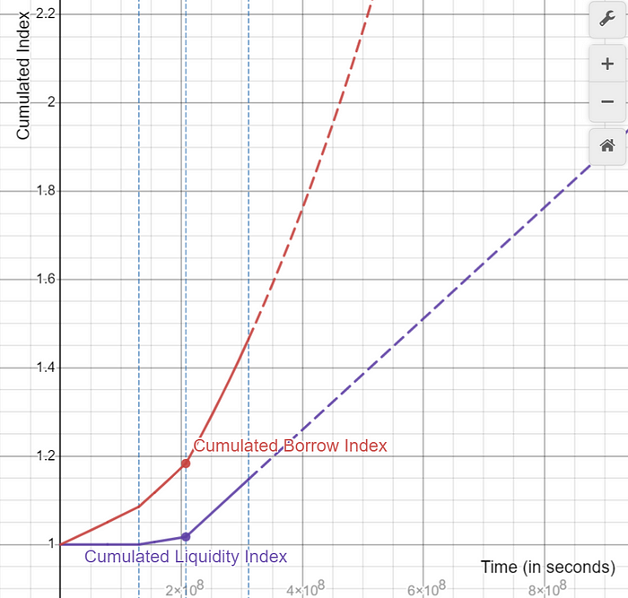
Since we have used the simple interest formula for cumulated liquidity index, the linear nature of the curve is expected. Similarly, since we have used the compound interest formula for cumulated borrow index, the exponential nature of the curve is expected.
User Accounts
Now that we have built up the intuition and the theory, let’s calculate the amounts that each user can redeem or need to repay.
Before that, let’s calculate the cumulated indexes for where there is some borrow or deposit.
We will now calculate the total amounts that each user will receive when they redeem or the amount that each has to pay back.
User A
Let us use:
Sᵃ to represent the total supply of user A
Cᵃ to represent the last updated cumulated supply index of user A.
Since user A has first deposited 1 token at T=0.
We update:
Sᵃ = 1
Cᵃ = 1 [Cᵗ for T=0]
To calculate the amount that will be received by the user A at any time, we can simply perform (Cᵗ/ Cᵃ)*Sᵃ .
At T=80, Amount = (1.01732/1)*1 = 1.01732
At T=120, Amount = (1.1477/1)*1 = 1.1477
User B
Let us use:
Sᵇ to represent the total supply of user B
Cᵇ to represent the last updated cumulated supply index of user B.
Since user B has first deposited 2 tokens at T=0.
We update:
Sᵇ = 2
Cᵇ = 1 [Cᵗ for T=0]
To calculate the amount that will be received by the user B at any time, we can simply perform (Cᵗ/ Cᵇ)*Sᵇ .
For T=80, Amount = (1.01732/1)*2 = 2.03464
The update by user B is on T=80 where the user withdraw 1 token. So we update:
Sᵇ = 2.03464 - 1 = 1.03464
Cᵇ = 1.01732 [Cᵗ for T=80]
Again let’s calculate the amount that the user will receive at time T=120.
Amount = (1.1477/1.01732)*1.03464 = 1.1672
User C
Let us use:
Sᶜ to represent the total supply of user C
Cᶜ to represent the last updated cumulated supply index of user C.
Since user C has first deposited 2 tokens at T=0.
We update:
Sᶜ = 2
Cᶜ = 1 [Cᵗ for T=0]
To calculate the amount that will be received by the user C at any time, we can simply perform (Cᵗ/ Cᶜ)*Sᶜ .
For T=80, Amount = (1.01732/1)*2 = 2.03464
The update by user C is on T=80 where the user deposits additional 1 token. So we update:
Sᵇ = 2.03464+1 = 3.03464
Cᵇ = 1.01732 [Cᵗ for T=80]
Again let’s calculate the amount that the user will receive at time T=120.
Amount = (1.1477/1.01732)*3.03464 = 3.4235
User D
Let us use:
Vᵈ to represent the total borrows of user D
Bᵈ to represent the last updated cumulated borrow index of user D.
Since the user D first borrowed 1 token at T=50.
We update:
Vᵈ = 1
Bᵈ = 1.085664 [Bᵗ for T=50]
To calculate the amount that needs to be repaid by user D at any time, we can simply perform (Bᵗ/ Bᵈ)*Vᵈ .
For example, at T=80, Amount = (1.18352/1.085664)*1 = 1.09013
Again let’s calculate the amount that the user has to repay at T=120.
Amount = (1.465493/1.085664)*1 = 1.34986
User E
Let us use:
Vᵉ to represent the total borrows of user E
Bᵉ to represent the last updated cumulated borrow index of user E.
Since user E first borrowed 2 tokens at T=80.
We update:
Vᵉ = 2
Bᵉ = 7.5547323 [Bᵗ for T=80]
To calculate the amount that needs to be by user E at any time, we can simply perform (Bᵗ/ Vᵉ)*Lᵉ .
Let’s calculate the amount that the user has to repay at T=120.
Amount = (1.465493/1.18352)*2 = 2.47649
Scaled Amount
For the calculation of the total amount that a user can redeem or should repay we made use of the cumulated indices. The total amount that user A, can redeem can be calculated with:
Total Amount = (Cᵗ/ Cᵃ)*Sᵃ
Where,
Sᵃ is the actual amount deposited by user A
Cᵃ is the last updated cumulated supply index of user A.
We can adjust the above formula such that
Total Amount = (Sᵃ/ Cᵃ)*Cᵗ
The scaled liquidity amount is the value obtained by dividing the actual amount deposited by the cumulated index at the time of deposit i.e. last updated position. If we denote the scaled liquidity amount for user A by sᵃ, then the scaled liquidity amount for user A can be defined as sᵃ = (Sᵃ/ Cᵃ)
To calculate the total amount that a user can redeem at any time, we can multiply the scaled liquidity amount of the user with the cumulated liquidity index at that time.
Similarly, scaled borrowed amount is the value obtained by dividing the actual amount borrowed by the borrow cumulated index at the time of borrow. If we denote the scaled borrowed amount for user D by vᵈ, then the scaled borrowed amount for user D can be defined as:
vᵈ = (Vᵈ/ Bᵈ), where
Vᵈ is the actual amount borrowed by user D
Bᵈ is the last updated cumulated borrow index of user D.
To calculate the total amount that a user has to repay at any time, we can multiply the scaled borrowed amount of the user with the cumulated borrow index at that time.
Total Borrows and Total Liquidity
Now that we have introduced the concept of scaled amount, we can revisit the total borrows and total liquidity that we talked about in the earlier part of this article. And this time, we consider the interest on the borrowed amount.
Let bₜ denote the total scaled borrows. Then the total borrows Bₜ at any time t can be calculated by multiplying bₜ with Bᵗ at that time.
Note: Do not confuse Bᵗ and Bₜ
Bᵗ is the cumulated liquidity index
Bₜ is the total borrows
Total Liquidity (Lₜ)= Available Liquidity (Lₐ)+ Total Borrows (Bₜ)
We can see how the total borrows and total liquidity change with time with the graph below.
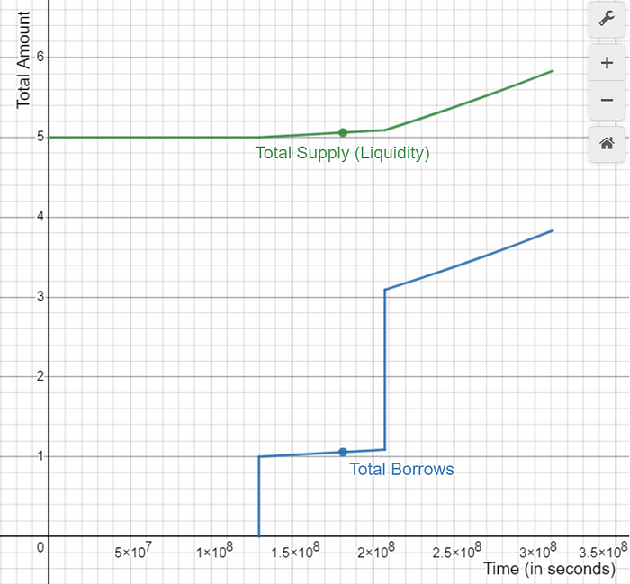
In the above graph, we can see that the difference between the total supply and total borrows is always the available liquidity. Since the available liquidity does not change without the deposit/borrow/redeem action, it is constant within the time intervals.
Since total borrows and total supply is changing with time, utilization rate also changes with time.
Let’s also plot the borrow rate and liquidity rate over time.
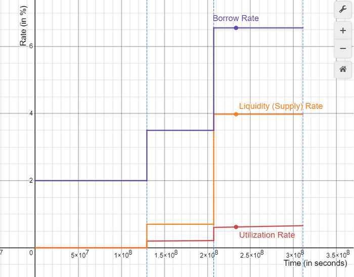
Note: Borrow rate and liquidity rate have not changed over time intervals, unlike the utilization rate. This is because the interest rates only change with deposit, borrow, redeem or repay event in the money market.
Calculations
At T=0
Since there can be no update prior to T=0, we set Cᵗ= C⁰ = 1. Similarly, Bᵗ = B⁰ = 1.
A deposits 1 token
Sᵃ=1
sᵃ=Sᵃ/Cᵗ=1
B deposits 2 tokens
Sᵇ=2
sᵇ=Sᵇ/Cᵗ=2
C deposits 2 tokens
Sᶜ=2
sᶜ=Sᶜ/Cᵗ=2
So,
Total Scaled Borrows bₜ = 0
Total Borrows Bₜ = bₜ*Bᵗ =0
Total Liquidity Lₜ= Lₐ + Bₜ =5
Utilization Rate U= Bₜ/Lₜ = 0
Borrow Rate Rᵥ= 2%
Liquidity Rate Rₗ = 0%
At T=50
Cᵗ=1. [Rₗ = 0% from T=0 to T=50]
Bᵗ = 1.08566 [Rᵥ= 2% from T=0 to T=50]
D borrows 1 token
Vᵈ = 1
vᵈ = Vᵈ/Bᵗ = 0.92108
Available Liquidity Lₐ= 4 [Since 1 token is borrowed]
So,
Total Scaled Borrows bₜ = 0.92108
Total Borrows Bₜ = bₜ*Bᵗ =1
Total Liquidity Lₜ= Lₐ + Bₜ =5
Utilization Rate U= Bₜ/Lₜ =0.2
Borrow Rate Rᵥ=3.5%
Liquidity Rate Rₗ = 0.7%
At T=80
Cᵗ=1.017326 [Rₗ = 0.7% from T=50 to T=80]
Bᵗ = 1.18352 [Rᵥ= 3.5% from T=50 to T=80]
B withdraws 1 token
Lₐ = 3
Since B had deposited previously, B can withdraw sᵇ * Cᵗ = 2.034652
Sᵇ = 2.034652–1 = 1.034652
sᵇ = Sᵇ/Cᵗ = 1.017326
C deposits an additional 1 token
Lₐ = 4
Sᶜ = 1
sᶜ = Sᶜ/Cᵗ = 0.9829
Since C had deposited 2 tokens previously, we add newly calculated sᶜ with the previous sᶜ.
Thus, sᶜ = 2.9829
E borrows 2 tokens
Lₐ = 2
Vᵉ = 2
vᵉ = Vᵉ/Bᵗ = 1.68987
So,
Total Scaled Borrows bₜ = 0.92108 + 1.68987 = 2.61087
Total Borrows Bₜ = bₜ*Bᵗ =3.09011
Total Liquidity Lₜ= Lₐ + Bₜ =5.09011
Utilization Rate U= Bₜ/Lₜ =0.60708
Borrow Rate Rᵥ=6.5531%
Liquidity Rate Rₗ = 3.978%
At T=120
Cᵗ=1.15037 [Rₗ = 3.978% from T=80 to T=120]
Bᵗ = 1.46805 [Rᵥ= 6.551% from T=80 to T=120]
So,
Total Scaled Borrows bₜ = 2.61087
Total Borrows Bₜ = bₜ*Bᵗ =3.83288
Available liquidity Lₐ = 2
Total Liquidity Lₜ= Lₐ + Bₜ =5.83288
User A can redeem sᵃ*Cᵗ = 1.15037
User B can redeem sᵇ*Cᵗ = 1.17030
User C can redeem sᶜ*Cᵗ = 3.43143
User D has to repay vᵈ * Bᵗ = 1.352191
User E has to repay vᵉ * Bᵗ = 2.48081
At T=240
Cᵗ=1.6017 [Rₗ = 3.978% from T=120 to T=240]
Bᵗ = 2.8012 [Rᵥ= 6.551% from T=120 to T=240]
So,
Total Scaled Borrows bₜ = 2.61087
Total Borrows Bₜ = bₜ*Bᵗ =7.313569
Available liquidity Lₐ = 2
Total Liquidity Lₜ= Lₐ + Bₜ =9.313569
User A can redeem sᵃ*Cᵗ = 1.6017
User B can redeem sᵇ*Cᵗ = 1.6294
User C can redeem sᶜ*Cᵗ = 4.7777
User D has to repay vᵈ * Bᵗ = 2.5801
User E has to repay vᵉ * Bᵗ = 4.7336
Summary of Calculations
The calculations above have been summarized in the following spreadsheet as well.
Conclusion
The calculations above used a limited model using a single reserve. In practice, however, we have multiple reserves, each reserve having its own borrow rate, optimum utilization rate, and other constants. But the mathematical concepts that we have discussed here are the same for any number of reserves. Moreover, the understanding of these mathematics will be used in the implementation of smart contracts, which will be discussed in the final part of the three-part series.